After almost three decades of active research, short-term wind power forecasting is now considered a mature field. It has been widely and successfully put into operation within the 10 past years. Anticipating the amount of energy that’s to be harvested is key to load balancing and revenue generation for any productive wind farm, and two main approaches for wind power forecasting are usually considered in the literature (though are sometimes opposed): Physical and statistical.

Physical models tend to draw data from external numerical weather prediction (NWP) models, and include mesocale and computational fluid dynamics (CFD) modeling; whereas, statistical models employ different statistical algorithms. These include grey/black box statistical learning, phase/magnitude correction, and data filtering.

Over time, however, it’s been widely determined that an optimal combination of physical and statistical approaches are necessary to build a high-performance forecasting system.

Behind the optimal combination, there still resides a wide variety of design options. The following sheds some light on what performances one should expect from several modeling options for combining physics and statistics in wind forecasting. The case studies presented are taken from real wind farms in various climate and terrain conditions.

Usually, wind energy forecasting systems are classified along several axes:

·       Intraday/Extraday, or Short-term/Very short-term. This mode looks at the time ahead (i.e. horizon), from 0 to several hours for very short-term (intraday), and from some hours to some days for short-term (extraday);

·       Deterministic/Stochastic. These two opposite concepts use different scientific tools—physics and mechanics for a deterministic approach, as well as statistical tools and machine learning for stochastic approach;

·       Numerical weather prediction/Online data. There are basically two sources of data to perform wind power forecasting. The first one includes meteorological predictions, based on global measurements and advanced numerical computations; the second is online measurements, such as for instance, from supervisory control and data acquisition (SCADA) systems.

For each axis, one concept generally excludes the other. Intraday (very short-term) is commonly stochastic with online measurements, while extraday (short-term) is usually deterministic based on NWP data.

Therefore, the aim of the ideal wind forecasting tool is to breakdown these classifications by proposing a unique model, which merges all these techniques. A short-term forecasting solution has, in fact, been designed to take advantages of micro-scale CFD modeling and advanced statistical learning. In the frame of this model design, various options have been considered and evaluated, taking into account model performance and operational constraints (see Figure 1).

Deterministic forecast: A physical approach
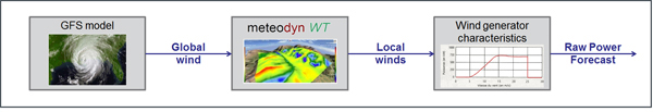A deterministic approach starts from a NWP, which predicts the meteorological wind over and around a wind farm area. Then, a computational fluid dynamics (CFD model) tool makes a micro-downscaling, so as to provide the future wind characteristics at the exact location of each turbine.

As a result of the measured power curves of the turbines, the air density provided by the numerical weather prediction and the planning maintenance (provided by the user), the final power output can be calculated. This step includes the interaction between the wind turbines, throughout the Jensen wake model. (Note: the Jensen model is, currently, one of the widely used wake models as it’s not only simple and easy to code, but also performs well on predicting wake loss.)

Machine learning: A stochastic approach
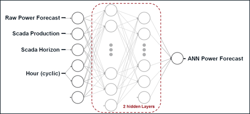The machine learning procedure is based on an artificial neural network (ANN). The architecture is a supervised, feed-forward and fully connected network. It’s trained using a back-propagation learning process, and selected thanks to a genetic algorithm (See Figure 2).

The optimization of input variables provides for the following final set:

·       Raw power forecast: The power provided by the deterministic approach;

·       SCADA production: The instant output power measured at the wind farm;

·       SCADA horizon: The time lag between the last measurement and the forecasted time;

·       Hour: The forecast time within the day (taking into account the night/day effects, which may be omitted in the deterministic approach).

Selecting data: Which to use?
A usual question raised in machine learning involves the historical data necessary to train the network. In this case, the historical NWP meteorological data has to be collected, along with long-term measurements at the wind farm site (i.e. observations).

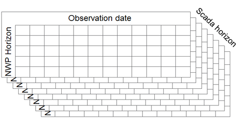
An automatic batch for re-running the deterministic approach provides the raw power forecast historical data. Herein, the NWP runs are provided twice a day and they cover several days. This provides several forecasts for each time step, with distinct NWP-horizons. But, to provide a match with the observations and measured data, a two-dimensional vision of time has to be adopted: Observation time versus NWP-horizon (see Figure 3).

With the addition of online measurements including each horizon, this two-dimensional vision of time must, then, be changed in a 3D time vision: Observation time versus NWP-horizon versus SCADA-horizon. A single observation can be predicted with different combinations of NWP and SCADA horizons (see Figure 4).

This process replicates several times the same data, as a single measurement is duplicated along the NWP and SCADA-horizon axes, which makes a strong correlation between the different data points. Constructing the learning/test/validation by pure randomization results in data snooping, wherein the data within different sets are strongly correlated. One way to avoid this failure is to gather the data by day before randomly splitting it into different sets.

Validation
This approach has been tested on a large wind farm (99 MW, 66 WTG), which is on a complex terrain. There are four NWP runs a day, with a 15-minute time step, leading to 2.5 millions of data points (250 k = 37 days for validation; 750 k = 108 days in test set; and 1 M5 = 216 days in the learning set). The results are based on the normalized root mean square error (RNMSE), as binned by SCADA horizons. Results include one year of historical data.

Results obtained of the whole process were compared with those form simpler approaches:

·       Pure persistence (forecasted power = measured power);

·       Persistence + ANN learning;

·       Pure NWP/CFD (with no calibration at all); and

·       NWP/CFD + ANN.

Conclusion
For horizon of less than 30 minutes, raw persistence is still preferred. For all longer horizons, the full model has a smaller error than other solutions. Numerical solutions (NWP/CFD) beat online measurements after three to four hours.

As can be seen, an optimal combination of physical and statistical forecasting models are necessary to build a reliable, high-performance wind forecasting system.

References for this article are available upon request.

Meteodyn provides wind resource assessment and integrated forecasting tools to wind farm operators, which now cover extra-day as well as intra-day power forecast.

Meteodyn
www.meteodyn.com