Page 21 - North American Clean Energy January February 2015

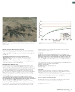
Figure 5. Example of a real wind farm site, which is situated in complex terrain, that’s been Figure 6. he root mean squared error (RNMSE) as a function of horizon scale
studied for a year

Machine learning: A stochastic approach
strongly correlated. One way to avoid this failure is to gather the data by day before
he machine learning procedure is based on an artiicial neural network (ANN). he randomly splitting it into diferent sets.
architecture is a supervised, feed-forward and fully connected network. It’s trained

using a back-propagation learning process, and selected thanks to a genetic algorithm Validation
(See Figure 2).
his approach has been tested on a large wind farm (99 MW, 66 WTG), which is on a
complex terrain. here are four NWP runs a day, with a 15-minute time step, leading to 2.5
he optimization of input variables provides for the following inal set:
millions of data points (250 k = 37 days for validation; 750 k = 108 days in test set; and

• Raw power forecast: he power provided by the deterministic approach;
1 M5 = 216 days in the learning set). he results are based on the normalized root mean
• SCADA production: he instant output power measured at the wind farm;
square error (RNMSE), as binned by SCADA horizons (see Image 5). Results include one
• SCADA horizon: he time lag between the last measurement and the forecasted time; year of historical data.
• Hour: he forecast time within the day (taking into account the night/day efects,

which may be omitted in the deterministic approach).
Results obtained of the whole process were compared with those form simpler approaches:
• Pure persistence (forecasted power = measured power);
Selecting data: Which to use?
• Persistence + ANN learning;
A usual question raised in machine learning involves the historical data necessary
• Pure NWP/CFD (with no calibration at all); and

to train the network. In this case, the historical NWP meteorological data has to be • NWP/CFD + ANN.
collected, along with long-term measurements at the wind farm site (i.e. observations).
An automatic batch for re-running the deterministic approach provides the raw Conclusion

power forecast historical data. Herein, the NWP runs are provided twice a day and For horizon of less than 30 minutes, raw persistence is still preferred. For all longer
they cover several days. his provides several forecasts for each time step, with distinct horizons, the full model has a smaller error than other solutions. Numerical solutions
NWP-horizons. But, to provide a match with the observations and measured data,
(NWP/CFD) beat online measurements after three to four hours.
a two-dimensional vision of time has to be adopted: Observation time versus NWP- As can be seen, an optimal combination of physical and statistical forecasting models are

horizon (see Figure 3).
necessary to build a reliable, high-performance wind forecasting system.
With the addition of online measurements including each horizon, this two-
dimensional vision of time must, then, be changed in a 3D time vision: Observation References for this article are available upon request.
time versus NWP-horizon versus SCADA-horizon. A single observation can be predicted

with diferent combinations of NWP and SCADA horizons (see Figure 4).
Meteodyn provides wind resource assessment and integrated forecasting tools to wind farm
his process replicates several times the same data, as a single measurement is operators, which now cover extra-day as well as intra-day power forecast.
duplicated along the NWP and SCADA-horizon axes, which makes a strong correlation
between the diferent data points. Constructing the learning/test/validation by pure Meteodyn | www.meteodyn.com

randomization results in data snooping, wherein the data within diferent sets are

North American Clean Energy 21